StatsCosmos: July 2016

This post is designed for a joint installation of Apache Hadoop 2.6.0, MongoDB 2.4.9, Apache Spark 1.5.1 (pre-built for Hadoop) and Ubuntu 14.04.3 LTS. The purpose of the illustration is to show how one can construct and summarize a database of the Last.fm social system profiles for the GroupLens HetRec 2011 Last.fm dataset using the Go Programming Language. The methodology is that outlined in Cantador, Bellogin and Vallet (2010).

The approach involves implementing the MapReduce programming model using a mapper-reducer set extracted from a Go word count application. The specific HetRec 2011 Last.fm dataset is the assignments dataset. The approach involves counting four assignment categories. These are as follows.

Assignments made by each user (using all tags)
Assignments made to each artist (using all tags)
Assignments made by each user with a specific tag
Assignments made to each artist with a specific tag

The results of the counting exercise can then be used to construct the six core social tagging system measures outlined in the paper. The measures can, in turn, be used to construct the social tagging system profiles outlined in the paper.

1. Model

In social tagging systems, one has a folksonomy defined as a tuple ℱ = {T,U,I,A}, where T = {t₁,…,t_L} is the set of tags, U = {u₁,…u_L} the set of users, I = {i₁,…,i_L} the set of items annotated with the tags of T and A = {(u_m,t_l,i_n)} ∈ U ⨯ T ⨯ I is the set of assignments (annotations) of each tag t_l to an item i_n by a user u_m.

In these systems, the users create or upload content (items), annotate it with the tags and share it with other users. The whole set of tags then constitutes a collaborative classification scheme. The classification scheme can then be used to search for and discover items of interest.

In the system the users and items can be assigned profiles defined as weighted lists of social tags. Generally, a user will annotate items that are relevant for them, so the tags she or he provides can be assumed to describe her/his interests, tastes and needs. It can additionally be assumed that the more a tag is used by a user the more important the tag is for her or him.

Similarly, the tags that are assigned to an item usually describe its contents. Consequently, the more users annotate the item with a particular tag the better the tag describes the item’s contents. It is important, however, to keep in mind a key feature of the assumptions. If a particular tag is used very often by users to annotate many items, then it may not be useful when one wants to discern informative user preferences and item features.

The above constructs and assumptions allow one to formulate a social tagging system recommendation problem that can be used as the basis for the analysis. Adomavicius and Tuzhilin (2005) formulate the recommendation problem as follows.

Let U = {u₁,…,u_M} be a set of users, and let I = {i₁,…,i_N} be a set of items. Let g: U ⨯ I → ℛ, where ℛ is a totally ordered set, be a utility function such that g(u_m,i_n) measures the gain of usefulness of item i_n to user u_m.

Then, what is desired is to choose for each user u ∈ U a set of items i ^max,u ∈ I, unknown to the user, which maximize the utility function g:

∀ u ∈ U, i ^max,u = arg max _{i ∈ I} g(u,i).

In content-based recommendation approaches g() is then formulated as follows.

g(u_m,i_n) = sim(ContentBasedUserProfile(u_m), Content(i_n)) ∈ ℜ^k, where

ContentBasedUserProfile(u_m) = u_m = (u_m,1,…, u_m,K) ∈ ℜ^k is the content-based user preferences of user u_m(namely, the content features that describe the interests, tastes and needs of the user).
Content(i_n) = i_n= (i_n,1,…,i_n,K) ∈ ℜ^k is the set of content features characterizing item i_n.

The ContentBasedUserProfile() and Content() descriptions are usually represented as vectors of real numbers (weights). In the vector representation each component in the tuple measures the “importance” of the corresponding feature in the user and item representations. The function sim() quantifies the similarity between a user profile and an item profile in the content feature space. This set up then allows one to develop approaches to determine the basket of items i ^max,u in the problem.

The approach taken in the paper (Cantador, Bellogin and Vallet, 2010) and this illustration is to consider the social tags in such systems as the content features that describe both the user profile and the item profile. This allows one to study the different weighting schemes that can be used to measure the “importance” of a given tag for each user and item. These weighting schemes result in the social tagging content-based Profile models (from the paper) that we will consider in this illustration.

Given the above modelling structure and formulation of the folksonomy, the simplest way of defining the profile of user u_m, is as a vector u_m = (u_m,1,…,u_m,L), where u_m,l= |{(u_m,t_l,i) ∈ A | i ∈ I}| is the number of times the user has annotated items with tag t_l. In an analogous manner, the item profile of i_n can be defined as a vector i_n= (i_n,1,…,i_n,L), where i_n,l= |{(u,t_l,i_n) ∈ A | u ∈ U}| is the number of times the item has been annotated with tag t_l.

The paper (Cantador, Bellogin and Vallet, 2010) extends these two definitions of user and item profiles by using different expressions for the vector component weights.

The formulation and modelling structure result in the following table of core elements in the profile and recommendation models proposed in the paper (Cantador, Bellogin and Vallet, 2010).

The elements can be used to define three profile models that we will consider in this illustration. These are the TF Profile Model, the TF-IDF Profile Model and the Okapi BM25 Profile Model.

TF Profile Model

The TF Profile Model results from the simple approach to define user and item profiles.

Essentially, one can count the number of times a tag has been used by a user or the number of times a tag has been used by the community to annotate an item. This information is available for the Last.fm system if one defines the artist songs as the items and the user_taggedartists dataset (assignments dataset) with the second and third columns interchanged as the A set in the analysis.

The profile model for user u_m = u(m) then consists of the vector u_m= (u_m,1,…,u_m,L), where u_m,l= tf_u(m)(t_l).

The profile for item i_n = i(n) is then similarly defined as the vector i_n= (i_n,1,…,i_n,L), where i_n,l= tf_i(n)(t_l)

TF-IDF Profile Model

The second profile model that is proposed in the paper is the TF-IDF profile model.

The proposed model is formulated as follows.

u_m,l = tfiuf_u(m)(t_l) = tf_u(m)(t_l)iuf(t_l)

i_n,l= tfiif_i(n)(t_l) = tf_i(n)(t_l)iif(t_l).

Okapi BM25 Profile Model

The third profile model proposed in the paper is the Okapi BM25 model which follows a probabilistic approach.

The model is formulated as follows.

where b and k₁ are set to the standard values of 0.75 and 2, respectively.

One of the aims of this illustration is to show how one can quantify the six social tagging system measures in the Table for the Last.fm social tagging system using the GroupLens HetRec 2011 Last.fm dataset.

2. Prepare the data

The approach that will be followed will involve creating key datasets that will serve as inputs to the MapReduce implementation. This will involve creating four datasets from which to compile the measures.

The first dataset will use the first column of the assignment dataset as the keys. The second will use the second column. The third will use an index created with the first and third columns. The fourth will use an index created with the second and third columns. The values to the keys are created in the mapping phase when the data is processed in Hadoop, MongoDB and Spark (using Go for Hadoop and Spark). The reduce phase in the processing will generate the core measures.

The MapReduces will thus produce datasets with which to quantify the first, second, fifth and sixth measures directly. The number of observations in the fifth and sixth output datasets will provide the numerator values for the third and fourth measures, respectively. The first and second datasets will provide the inputs for the calculation of the denominators for the third and fourth measures, respectively.

The resulting quantifications will then be used to formulate the profile models for each user and each artist.

3. Prepare the Mapper-Reducer set (experimental/under development)

The approach to the MapReduce will be to use a word count application prepared in Go. The source Go word count application was prepared by Damian Gryski and posted on Github on November 2, 2012. In this illustration minor modifications were made to the code in order to allow the resulting application to read the (generated) user, artist, artist-tag and user-tag indexes from the datasets.

The wordcount application was prepared using the dmrgo library. The dmrgo library is a Go library for use with the Hadoop Streaming protocol and is thus ideal for MapReduce using Hadoop Streaming and the Spark Pipe facility. The guide to the library provides the information required to create and run the MapReduces in this illustration. The instructions include how to include the mapper-reducer code in one’s scripts and most importantly, how to build the word count application.

The code for the application for this illustration was prepared using this Go programming tutorial, this Go tour and is as follows.

The Go application can be saved in a local system folder , < Local System Go Application Folder>. The basic approach for including the scripts in the applications (and the program) is to create the following two bash files and save them in local system folders. In the remainder of the illustration the bash files are treated as the mapper and the reducer.

4. Process the data in Hadoop, MongoDB and Spark

Hadoop Streaming

The first MapReduce can be implemented in Hadoop using the Hadoop Streaming facility. The commands for customizing the Hadoop run can be found in this tutorial.
In order to conduct the first MapReduce the following arrangements need to be made.

Input data file: InputData.txt

Hadoop Distributed File System (HDFS) input data folder: < HDFS Input Data Folder>

Local system Hadoop Streaming jar file folder: <Local System Hadoop Streaming jar File Folder>

Hadoop Streaming jar file: hadoop-streaming-2.6.0.jar

Local system mapper folder: <Local System mapper Folder>

Local system reducer folder: <Local System reducer Folder>

Local system mapper bash file: Mapper.sh

Local system reducer bash file: Reducer.sh

HDFS Output data folder: <HDFS Output Data Folder>

The next step is to run the following command on Ubuntu 14.04.3.

These are the contents of the resulting output file.

MongoDB

The four MapReduces can be implemented in MongoDB. The first step is to import the four datasets into MongoDB using mongoimport. The dataset can be called LastFM. The collections can be named as follows.

MapReduce one: User Tags
MapReduce two: Artist Tags
MapReduce three: User Profile
MapReduce four:Artist Profile

The collections can be viewed using the db.<LastFM collection>.find().pretty() command. For example, to view the input collection for the third MapReduce one can switch to the LastFM dataset. One can then use the db.UserProfile.find().pretty() to view the UserProfile collection.

The other collections can be viewed analogously.

The next step is to run the following program in order to run the MapReduce for the user tag counts.

Then one can run the db.UserTags_Counts.find().pretty() method to view the results.

It is also possible to use the method to run individual queries. For example to find the results for user 2 and tag 13 one can run db.UserTags_Counts.find({"_id": “2;13;”}).pretty() method.

The results can be run analogously for the other collections. The find().pretty() method will yield the following results for the MapReduces for the remainder of the collections.

The next step is to run the second MapReduce using PySpark.

PySpark (application)

The second MapPreduce can be implemented in the Spark Pipe facility using a PySpark application. The application can also include SQL queries from Spark SQL and NoSQL queries from MongoDB (PyMongo and rmongodb). The PyMongo query can be included in the application. The rmongodb script can be saved in a separate file.

In order to conduct the second MapReduce and generate the queries the following arrangements need to be made.

Input data file: InputData.txt

Local system input data folder: <Local System Input Data Folder>

Local system mapper folder: <Local System mapper Folder>

Local system reducer folder: <Local System reducer Folder>

Local system output data folder: <Local System Output Data Folder>

Local system mapper bash file: Mapper.sh

Local system reducer bash file: Reducer.sh

MongoDB instance: Have a MongoDB instance with the arrangements outlined in the MongoDB illustration

Local system rmongodb query Script Folder: <Local system PySparkQueryScript Folder>

PySpark query script: PySparkQueryScript.R

The PySpark Pipe application and the query script can be prepared using the tutorials in this post, the Spark Quick Start website, this Spark Guide, this post, this post, this post and this post. The application and query script are as follows.

The application and the script can be saved in appropriate local system folders. The application can be run using the bin/spark-submit script.

The application will generate the following output file contents, statistical summary measures, Spark SQL query and NoSQL MongoDB query.

What just happened? The PySpark application conducted the second MapReduce and wrote the results to file as shown in the first image. The application then took the in-memory results, created an SQL data frame and showed us the dataframe as shown in the second image. The application then took the second column in the dataframe, calculated statistical summary measures and showed us the results as shown in the third image.

The application then made a connection with MongoDB using PyMongo in the local machine, conducted a MapReduce on the ArtistTags collection from the MongoDB illustration and generated a results MongoDB collection on the LastFM database called PyMongoresults1. The application then read 10 records from the collection and printed the ten records on screen as shown in the first ten JSON entries in the last image. The application then generated two individual JSON queries from the PyMongoresults1 collection for artist-tag combinations 10002;127; and 10005;5770;. These two were also printed on screen. These are the next two JSON entries in the last image.

The application then called an R script which also made a connection with MongoDB using rmongodb. The script then made two queries. The first query was for User 2 from the UserProfile collection in the LastFM database. The second was for Artist 52 in the ArtistProfile collection in the LastFM database. The script then closed the connection (NULL entry) and returned the results to the application. The application took the results (two JSON queries and the NULL entry) from the R script and printed them on screen. These are the last two JSON entries and the NULL entry in the last image.

The next step is to run the third MapReduce using SparkR.

SparkR (application)

The third MapReduce can be implemented in the Spark Pipe facility using a SparkR application. The application can also include SQL queries from Spark SQL and NoSQL queries from MongoDB (PyMongo and rmongodb). The rmongodb query can be included in the application. The PyMongo script can be saved in a separate file.

In order to conduct the second MapReduce and generate the queries the following arrangements need to be made.

Input data file: InputData.txt

Local system input data folder: < Local System Input Data Folder>

Local system mapper folder: <Local System mapper Folder>

Local system reducer folder: <Local System reducer Folder>

Local system output data folder: <Local System Output Data Folder>

Local system mapper bash file: Mapper.sh

Local system reducer bash file: Reducer.sh

MongoDB instance: Have a MongoDB instance with the arrangements outlined in the MongoDB illustration

Local system SparkR query Script Folder: <Local System SparkRQueryScript Folder>

SparkR query script: SparkRQueryScript.py

Local system qplot folder: <Local System Qplot Folder>

Local system qplot Histogram .png file: Qplot.jpeg

The SparkR Pipe application and the query script can be prepared using the tutorials in this post, the Spark Quick Start website, this Spark Guide, this post, this post , this post, this post and this post. The application and the supporting script are as follows.

The application and the script can be saved in appropriate local system folders. The application can be run using the bin/spark-submit script:

The application will generate the following output file contents, qplot Histogram .jpeg file, Spark SQL query, statistical summary measures and NoSQL MongoDB query.

What just happened? The SparkR application ran the third MapReduce and wrote the results to file as shown in the first image. The application then took the second column from the RDD, generated a Histogram using the qplot function and also saved it to a file. This is the graph in the second image. The application then took the in-memory data and used it to create an SQL data frame. The application then showed the dataframe as shown in the third image.

The application then took the second column in the dataframe, calculated statistical summary measures and showed us the results as shown in the fourth image. The application then established a connection with MongoDB using rmongodb in the local machine (indicated by the TRUE) and generated two JSON queries. The first was a query on the UserTags collection (in the MongoDB illustration) for user-tag combination 2;13;. The second was query on the ArtistProfile_id_Counts collection for artist 52. The application then printed the results of the queries on screen. These are the first two JSON entries in the last image. The application then closed the connection which is indicated by the NULL entry in the last image.

The application then called a SparkRQuery python script. The script made a connection with the MongoDB LastFM UserProfile collection on the local machine. The Python script conducted a MapReduce on the UserProfile collection from the MongoDB illustration (using PyMongo) and generated a results collection called PyMongoresults2 in the LastFM database.

The script then read 10 records from the collection and made two queries. The first query was basic and the second was specific. The basic query used the PyMongo find_one() method. The specific query also used the find_one() method but used the specific document functionality. The specific query was for user 52.

The script then made a connection with the PyMongoresults1 collection from the PySpark PyMongo MapReduce and made two queries. The two queries were similar to the preceding two queries in that the first was basic (using find_one()) and the second was specific (also using find_one()). The second query was for the artist-tag combination 10002;12051;. The script then returned the 14 JSON queries to the application. The application printed the results on screen as shown in the last image.

The next step is to conduct the fourth MapReduce in the Scala Spark-shell.

Scala Spark-shell program

The fourth MapReduce can be run in the Spark Pipe facility in a Scala Spark-shell program. The shell program can also include SQL queries from Spark SQL and NoSQL queries from MongoDB (PyMongo and rmongodb). The rmongodb and PyMongo scripts can be saved in separate files.

In order to run the fourth MapReduce and generate the queries the following arrangements need to be made.

Input data file: InputData.txt

Local system input data folder: <Local System Input Data Folder>

Local system mapper folder: <Local System mapper Folder>

Local system reducer folder: <Local System reducer Folder>

Local system output data folder: <Local System Output Data Folder>

Local system mapper bash file: Mapper.sh

Local system reducer bash file: Reducer.sh

MongoDB instance: Have a MongoDB instance with the arrangements outlined in the MongoDB illustration

Local system rmongodb query Script Folder: <Local system rmongodb query Script Folder>

Local system PyMongo query Script Folder: <Local system PyMongo query Script Folder>

rmongodb query script: ScalaSparkShellrmongodbScript.R
PyMongo query script: ScalaSparkShellPyMongoScript.py

The Scala Spark-shell Pipe program and the query script can be prepared using the tutorials in this post, the Spark Quick Start website, this Guide, this post, this post and this post. The program and scripts are as follows.

The program will generate the following output file contents, Spark SQL query, statistical summary measures and NoSQL MongoDB query.

What just happened? In the Scala Spark-shell program the fourth MapReduce was run and the results were written to a file. The contents of the file are shown in the first image. The results were then used to create an SQL data frame and show it. This part of the program will result in the output shown in the second image.

The next part of the program then takes the second column in the dataframe, calculates statistical summary measures and asks Spark to show the results. This part of the program will result in the output shown in the third image.

The next part of the program then calls an R script which makes a connection with MongoDB using rmongodb on the local machine and makes two JSON queries from the LastFM database. The first is on the UserTags_Counts collection for user-tag combination 2;13;. The second is on the ArtistProfiles_id_Counts collection for artist 52. The script then closes the connection, returns the results to the program and puts them to a Scala string variable called rmongoquery. The contents are shown on the fourth image (print statement).

The next part of the program then calls a Python script. The Python script makes a connection with the MongoDB ArtistProfile collection in the LastFM database.
The script then runs a MapReduce on the collection and generates a LastFM database collection called PyMongoresults3. The script then reads 10 records from the collection, conducts a basic find_one() query and a specific query for artist 52.

The script returns the results to Spark and they are put into a string variable called pymongoquery. The program then prints the contents of the variable in screen. This is shown in the last image.

This sequence can run run analogously using a Spark Java application.

Java Spark (application)

The fourth MapReduce can also be run in the Spark Pipe facility in a Spark Java application. The application can also include SQL queries from Spark SQL and NoSQL queries from MongoDB (PyMongo and rmongodb). The rmongodb and PyMongo scripts can be saved in separate files.

In order to conduct the fourth MapReduce and generate the queries the following arrangements need to be made.

Input data file: InputData.txt

Local system input data folder: <Local System Input Data Folder>

Local system mapper folder: <Local System mapper Folder>

Local system reducer folder: <Local System reducer Folder>

Local system output data folder: <Local System Output Data Folder>

Local system mapper bash file: Mapper.sh

Local system reducer bash file: Reducer.sh

MongoDB instance: Have a MongoDB instance with the arrangements outlined in the MongoDB illustration

Local system rmongodb query Script Folder: <Local System SparkJavaQueryRscript Folder>

Local system PyMongo query Script Folder: <Local System SparkJavaQueryPythonscript Folder>
rmongodb query script file: SparkJavaQueryRScript.R

PyMongoDB query script file: SparkJavaPythonScript.py

JavaScriptSubmit bash file: SparkJavaQueryScriptsSubmit.sh

The Java Spark Pipe application and query scripts can be prepared using the tutorials in this book, this book, the Spark Quick Start website, this Spark Guide, this post, this post, and this post. The query script can be called from the Java application using a bash file which one can name JavaScriptSubmit.sh. The application, bash file and query scripts are as follows.

The application java file can be exported to a jar file. The jar file, bash file and scripts can be saved in appropriate local system folders. The application can be run using the bin/spark-submit script.

The application will generate the following output file contents, Spark SQL query and NoSQL MongoDB query.

What just happened? The application ran the fourth MapReduce and wrote the results to file whose contents are shown in the first image. The application then created a dataframe containing the in-memory results. The application then ran an SQL query on the dataframe for artist 52 and printed the results on screen. These are the first two entries in the last image.

The application then called a bash query submit script to conduct two MongoDB queries. The bash query submit script calls two scripts, a rmongodb query script and a PyMongo query script. The rmongodb query is run first. The rmongodb query script makes a connection with MongoDB on the local machine. The script then runs two queries in the LastFM database. The first query is on the UserTags_Counts collection for user-tag combination 2;13;. The second is on the ArtistProfile_id_Counts collection for artist 52. The script then closes the connection and takes the results to bash. Bash in turn prints the results returned to screen.

The bash query script then calls the PyMongo query script. The PyMongo query script also makes a connection with MongoDB on the local machine. The script then makes a connection with the ArtistProfile collection in the LastFM database and conducts a MapReduce that computes the artist profile sizes.

The results of the MapReduce are written to a LastFM collection called PyMongoresults3 in MongoDB. The script prints ten records from the database. It then conducts a basic query using the find_one() method on the PyMongoresults3 collection and prints the results. The script then conducts a specific query for artist 52 and prints the results. The printed results are taken to bash. Bash prints the results returned to screen.

The application prints all the output printed to screen by bash to screen in Spark as shown in the remaining entries in the last image.

5. Query the data

The data housed in MongoDB can additionally be queried using a ShinyMongo application from GitHub. The GitHub Gist also includes installation instructions and additional tutorials on Shiny Apps can be obtained from the Shiny tutorials.

The arrangement in this illustration requires Shiny, rmongodb, rjava, an instance of R and an instance of MongoDB (as outlined in the MongoDB illustration). The ShinyMongo application is available in downloadable form and in script form. The downloadable form can be run using the following commands in the R shell.

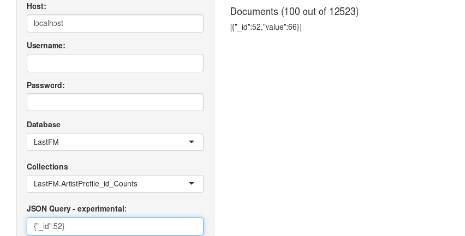
The command will launch the Shiny App. The graphical user interface has the following features.

The queries can be entered in the experimental JSON field and the size of the query is limited to 100 entries.

The application can be run locally using the ui.R and server.R scripts in the Gist (and following the Shiny tutorials). The Shiny App can be launched using the following commands in the R console.

In the case of the MongoDB (including rmongodb and PyMongo) part of the illustration the resulting locally based interface has the following features.

6. Analyze/Summarize the data using Histograms

The data can be further analyzed/summarized using the SGPlot Procedure in the SAS software. One can prepare a program using the tutorial in this post to generate the top 20 counts from MapReduce output data in turn. Suppose we have a Microsoft Excel dataset with the following structure.

One can then import the data into a SAS software work dataset, say, called import. If one runs the following code for <var> being UserID and chooses the first title option on line 8.

One will obtain the following plot.

The other plots can be generated similarly. In the case for <var>=ArtistID and appropriate dataset.

In the case for <var>=UserIDTagID, second title option on line 8 and appropriate dataset.

In the case for <var>=ArtistIDTagID, appropriate title option and appropriate dataset.

The next step is to obtain the statistical summary measures using the stat.desc() function in the pastecs package in R.

In the case of the user tags counts the statistical summary measures are as follows.

In the case of the artist tags counts.

In the case of the user profile counts (user profile size).

In the case of the artist profile counts (artist profile size).

The data can then be analyzed using Relative Frequency Histograms in R using the HistogramTools package. The histograms can be written to file using R grDevices.
The program has the following general structure for a numeric vector x.

The Relative Frequency Histograms for each of the output files from the MapReduces, the TF-IDF Profiles (user and artist) and the Okapi BM25 Profiles (user and artist) are as follows.

The user tags Relative Frequency Histogram.

The artist tags Relative Frequency Histogram.

The user profile Relative Frequency Histogram.

The artist profile Relative Frequency Histogram.

The user TF-IDF profile Relative Frequency Histogram.

The artist TF-IDF profile Relative Frequency Histogram.

The user Okapi BM25 profile Relative Frequency Histogram.

The artist Okapi BM25 profile Relative Frequency Histogram.

7. Conclusions

The illustration showed how one can construct social tagging system profile models for the Last.fm dataset using the profile models proposed in the paper Cantador, Bellogin and Vallet (2010). The results from the dataset are exciting as well as interesting. The resulting findings and constructions from the illustration can be used as inputs to an analysis of the dataset using the similarity measures proposed in the paper.

Interested in other posts on Big Data and Cloud Computing from the Stats Cosmos blog?

Check out my other posts