StatsCosmos: How to apply MapReduce to the Delicious dataset using Hadoop, MongoDB and Spark (Spark-shell, PySpark, Spark Applications, SparkR and SparkSQL)

This post is designed for a joint installation of Apache Hadoop 2.6.0, Apache Spark 1.5.1 (pre-built for Hadoop), MongoDB 2.4.9 and Ubuntu Server 14.04.3 LTS. This illustration shows how one can use MapReduce to construct metrics in content-based recommendation models for social tagging systems. The specific system is the GroupLens HetRec 2011 Delicious Bookmarks dataset system. The illustration is composed of two posts.

The theoretical framework is that outlined in the paper: Content-based Recommendation in Social Tagging Systems by Cantador, Bellogin and Vallet, published in 2010. The MapReduce implementation approaches are Hadoop Streaming, Spark WordCount (Scala program and Python Application), Spark Pipe (Scala program and Python Applications), Spark SQL (SparkR and Scala Spark-shell) and MongoDB. The core dataset is the Bookmark Assignments dataset which translates to a version of the A set in the paper.

The procedure translates to 17 MapReduce jobs which can be categorized into two phases. The first phase involves constructing the element definitions (and weights) in the paper and the second phase the utility metrics (similarity measures). The first phase is composed of four MapReduce jobs and will be outlined in this post.

The second phase is composed of the remaining jobs. The first two MapReduce jobs in the second phase involve constructing the first similarity measure (two metrics) and will also be outlined in this post. The remaining eleven MapReduce jobs will be outlined in the second post.

1. The Model

In a social tagging system (Cantador, Bellogin and Vallet, 2010), users create or upload content, annotate it with their own words and share it with other system users. The content is referred to as items and the annotations as tags. The tagging system is then an unstructured collaborative content classification system called a folksonomy. The classification system can then be used by system users to search for and discover items of interest.

The modeling of the system rests on two key assumptions. The first is that users will generally annotate items that are relevant for them and thus their tags can be seen to be a reflection of their interests, tastes and needs. It can additionally be assumed that the more a tag is used by a certain user, the more the important the tag is for them.

The second assumption is that tags assigned to items describe their contents. Similarly, the more a certain item is annotated with a particular tag, the better the tag describes the item’s contents.

It is important to keep in mind, however, that if a tag is used very often by users to annotate many items, it may not be useful to discern the information assumed.

A folksonomy ℱ can be defined mathematically as a tuple ℱ = {T, U, I, A}, where T = {t₁,......, t_L} is the set of tags, U = {u₁,......, u_M} is the set of users and I={i₁,......, i_N} is the set of items. A set A = {(u_m, t_l, i_n)} ∈ U * T * I is then the set of annotations, tag t_l to item i_n by user u_m.

The paper then outlines the following formulation of the recommendation problem according to Adomavicius and Tuzhilin (2005):

For a totally ordered set ℜ, one can define a utility function g, g: U * I ➙ ℜ, such that g(u_m,i_n) measures the gain of usefulness of item i_n to user u_m. The aim of the analysis is then, for each user u ∈ U, to find items i ^{max, u}∈ I, unknown to the user, that maximize g:

∀ u ∈ U, i ^{max, u}= arg max_i_∈Ig(u,i).

In the modeling framework of the paper, content-based recommendation approaches formulate g as the metric:

g(u_m,i_n) = Sim(ContentBasedUserProfile(u_m), Content(i_n)) ∈ ℜ, where,

ContentBasedUserProfile(u_m) = u_m = (u_m,l,........,u_m,K) ∈ ℝ^k, k ∈ ℕ, is the content-based preferences of user u_m (i.e. described in assumption one).
Content(i_n) = i_n = (i_n,l,........,i_n,K) ∈ ℝ^k, k ∈ ℕ, is the set of content features characterizing item i_n (i.e. described in assumption two).

The vectors can then be represented as vectors of real numbers, called weights, in which each array element provides a measure of the importance of the corresponding feature in the user and item model representations. The similarity function Sim() then computes the similarity between a user profile and the item profile in the content feature space.

The next critical component is then to consider the tags as the content features that describe both the user and item profiles (as per assumptions one and two). In our MapReduce formulation these descriptions are housed in the elements computed in the first phase.

These elements allow for the study of the weighting schemes outlined in the paper. The schemes are the TF Profile Model, TF-IDF Profile Model and the Okapi BM25 Profile Model.

The tag weighting schemes can then be used to construct the similarity (utility) functions. In our MapReduce formulation, this is the second phase.

The basic profile model defines the profile of user u_m as a vector
u_m = (u_m,1,........,u_m,L), where u_m,l = |{(u_m,t_l,i) ∈ A | i ∈ I}| is the number of times a user u_mhas annotated items with tag t_l.

The item profile of i_nis the vector i_n = (i_n,l,........,i_n,L), where i_n,l = |{(u,t_l,i_n) ∈ A | u ∈ U}| is the number of times item i_nhas been annotated with tag t_l.

The important point to note in this definition is that both the user and item profiles are defined from components of the A set, which can be constructed from the Bookmarkassignments dataset. In this illustration we use the simple formulation of defining the items to be the bookmarked URL's (in the Bookmarks file) in order to use the Bookmarkassignment dataset as our A set.

In the next step we use the methodology of the paper to define the other profile models from the basic profile model. These involve the following elements, which constitute phase one of our MapReduce approach.

The TF User and TF Item Profile

The TF User and TF Item Profiles can be constructed as follows.

TF User profile (user u_m and tag t_l)

TF Item profile (item i_n and tag t_l)

The TF-IDF User and TF-IDF Item Profile

The TF-IDF User and TF-IDF Item Profiles can be constructed as follows.

TF-IDF User profile (user u_m and tag t_l)

TF-IDF Item profile (item i_n and tag t_l)

Okapi BM25 User and Okapi BM25 Item Profile

The Okapi BM25 User and Okapi BM25 Item Profiles can be constructed as follows.

Okapi BM25 User Profile (user u_m and tag t_l)

Okapi BM25 Item Profile (item i_n and tag t_l)

The values b and k₁ are the standardized values, 0.75 and 2, respectively.

TF-based Similarity

In terms of the similarity measures, the TF-based similarity metrics that can be constructed from the basic model are as follows:

The similarity measures constitute the first two MapReduces in phase two. The maxima for scaling the measures can be obtained from the resulting files using Spark.

2. Prepare the data

The dataset used is the user_taggedbookmarks dataset and has the following columns:

userID
bookmarkID
tagID
day
month
year
hour
minute
second

The first three columns can be used to construct the A set entries. The dataset is composed of 437593 observation tuples (rows). The MapReduces generally involve constructing key indices using the columns of the A set (phase one) and key value pairs from the processed data (phase two). For example, for the first MapReduce, to determine the tag assignments by user u_m for each tag t_l (i.e. u_m,l ) we construct the index u_m;t_l; (from the first and third columns) and conduct Hadoop/Spark word count. This provides the u_m,l element in the paper elements.

An analogous approach can be followed for the i_n,l using the second and third columns to define the index i_n;t_l; and conduct Hadoop/Spark word count.

The fifth and sixth elements, namely, the user and item profile sizes (i.e. |u_m| and |i_n|, respectively) can be determined by defining the first and second columns, respectively, as the MapReduce keys (index) and conducting the Hadoop/Spark word counts. The output files from the word counts yield M, the number of users (in the A set) and N the number of items. One can then additionally, use the output files to construct avg(|u_m|) and avg(|i_n|) required for the Okapi BM25 Profile model weights.

The third and fourth elements, can be constructed using the M and N from the output files of the third and fourth MapReduce. The six components can then be used to construct the remaining Profile model weights. The components are then used as input components to the two sum MapReduce jobs that are used to construct the first two similarity measures.

3. Prepare the Mapper-Reducer sets

The Mapper-Reducer sets in the illustration are prepared in Ruby, Python, R and Perl.

Ruby mapper-reducer set

The Ruby mapper-reducer set was prepared using the tutorials in this post and this post.

Ruby mapper

Ruby reducer

Perl mapper-reducer set

The Perl mapper-reducer set was prepared using the tutorials in this post and this post.

Perl mapper

Perl reducer

R mapper-reducer set

The R mapper-reducer set was prepared using the tutorials in this gist and this post.

R mapper

R reducer

Python mapper-reducer set

The Python mapper-reducer set was prepared using the tutorials in this post and this post.

Python mapper

Python reducer

4. Process the data in Hadoop and Spark

PySpark WordCount Application

The first MapReduce (Simple PySpark Word Count Application) can conducted on a column of data composed of an index created using the first and third columns of the A set. In order to conduct the MapReduce the following arrangements should be made.

Input data file: InputData.txt

Local system input data folder: Local system Input Data Folder

Local system output folder: Local system Output Folder

Choose the data delimiter to be a space.

The following program, prepared using the tutorial in the Spark Examples website, can be saved in a Python file (SimplePysparkWCApp.py).

The MapReduce can be run using the following command in Ubuntu 14.04.3 obtained from the Spark Quick Start website.

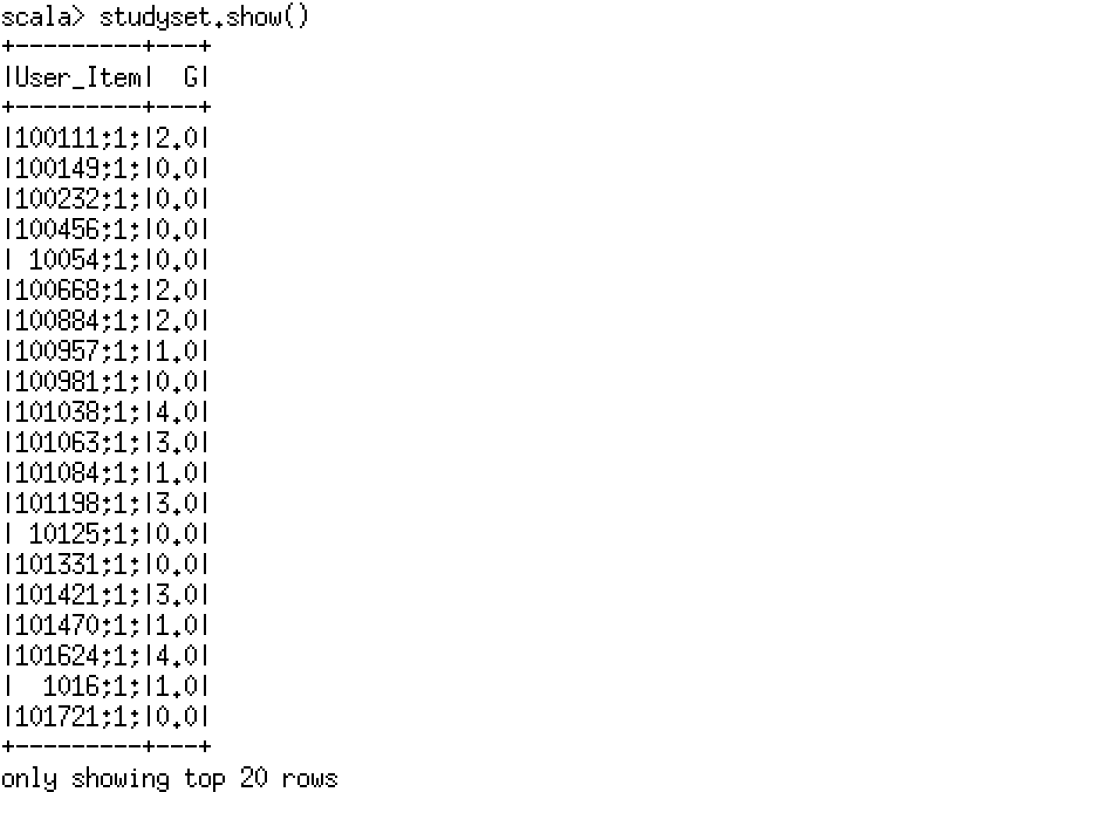
These are the contents of the output file.

Scala Spark-shell WordCount

The second MapReduce (Scala Spark-shell Word Count program) can be conducted on a column of data composed of an index created using the second and third columns of the A set. In order to conduct the MapReduce the following arrangements should be made.

Input data file: InputData.txt

Local system input data folder: Local system Input Data Folder

Local system output folder: Local system Output Folder

Choose the delimiter to be a space.

The following Simple program, prepared using the tutorial in the Spark Examples website can be run in the Scala Spark-shell (local mode on four cores).

These are the contents of the output file.

Hadoop Streaming (Ruby mapper-reducer set)

The third MapReduce (Ruby mapper-reducer set Hadoop Streaming) can be conducted on a column of data composed of an index created using the first column of the A set. In order to conduct the MapReduce it is necessary to make the following arrangements.

Input data file: InputData.txt

HDFS input data folder: HDFS Input Data Folder

HDFS output folder: HDFS Output Folder

Local system mapper folder: Local system mapper Folder

Local system reducer folder: Local system reducer Folder

Hadoop Streaming jar: hadoop-streaming-2.6.0.jar

Local system Hadoop Streaming jar folder: Local system Hadoop streaming jar Folder

Mapper file: Profile_mapper.rb

Reducer file: Profile_reducer.rb

Choose the delimiter to be a space.

The MapReduce can be run using the following command in Ubuntu 14.04.3.

These are the contents of the output file.

PySpark Pipe WordCount Application (Ruby mapper-reducer set)

The fourth MapReduce (Simple PySpark Pipe Word Count Application) can be conducted on a column of data composed of an index created using the second column of the A set. In order to conduct the MapReduce the following arrangements should be made.

Input data file: InputData.txt

Local system input data folder: Local system Input Data Folder

Local system output folder: Local system Output Folder

Local system mapper folder: Local system mapper Folder

Local system reducer folder: Local system reducer Folder

Mapper file: Profile_mapper.rb

Reducer file: Profile_reducer.rb

Choose the delimiter to be a space.

The following program, prepared using the tutorial in this post, the Databricks Guide/Tutorials on the book and the Spark Quick Start website, can be saved in a Python file (SimplePysparkPipeWCApp.py) in Ubuntu 14.04.3.

The MapReduce can be run using the following command in Ubuntu 14.04.3 obtained from the Spark Quick Start website.

These are the contents of the output file.

Hadoop Streaming (Python mapper-reducer set)

The fifth MapReduce (Hadoop Streaming) can be conducted on the outputs of the first MapReduce (i.e. u_m,lfrequencies) for user 8 summed over the non-zero i_n,lfor each item i_n. This can be achieved by attaching user 8’s u_m,l = f_{u_m}(t_l) (tag frequencies) to the non-zero i_n,lfor each tag t_lin the i_nprofiles. This is the method of Noll and Meinel (2007). The sums can then be scaled, in line with the methodology proposal in the paper (i.e. Cantador, Bellogin and Vallet, 2010), to values between 0 and 1 by dividing with the maximum numerator sum value.

In order to run the MapReduce the following arrangements need to be made.

Input data file: InputData.txt

HDFS input data folder: HDFS Input Data Folder

HDFS output folder: HDFS Output Folder

Local system mapper folder: Local system mapper Folder

Local system reducer folder: Local system reducer Folder

Hadoop Streaming jar: hadoop-streaming-2.6.0.jar

Hadoop Streaming jar folder: Local system Hadoop streaming jar Folder

Mapper file: Summapper.py

Reducer file: Sumreducer.py

Choose the delimiter to be a tab.

The MapReduce can be run using the following command in Ubuntu 14.04.3.

These are the contents of the output file.

PySpark Pipe Sum Application (Python mapper-reducer set)

The sixth MapReduce (Simple PySpark Pipe Sum Application) can be conducted on the outputs of the second MapReduce (i.e. i_n,lfrequencies) for item 1 summed over the non-zero u_m,lfor each user u_m. This can be achieved by attaching item 1’s i_n,l= f_{i_n}(t_l)(tag frequencies) to the non-zero u_m,lfor each tag t_lin the u_mprofiles. The sums can then be scaled, in line with the methodology proposal in the paper (i.e. Cantador, Bellogin and Vallet, 2010), to values between 0 and 1 by dividing with the maximum numerator sum value.

In order to run the MapReduce the following arrangements need to be made.

Input data file: InputData.txt

Local system input data folder: Local system Input Data Folder

Local system output folder: Local system Output Folder

Local system mapper folder: Local system mapper Folder

Local system reducer folder: Local system reducer Folder

Mapper file: Summapper.py

Reducer file: Sumreducer.py

Choose the delimiter to be a tab.

The MapReduce can be run using the following command in Ubuntu 14.04.3 obtained from the Spark Quick Start website.

These are the contents of the output file.

5. Check the results (Hadoop, MongoDB and Spark)

MongoDB

The first MapReduce can be checked by reading an index created using the first and third columns of the A set into MongoDB and conducting the MapReduce.

Once the data is in MongoDB one can run the following commands prepared using the tutorial in this post, to view the collection UserID_TagID in database Delicious.

UserID tag specific counts

The MapReduce for the User 8 tag 1 counts can be conducted by running the following program prepared using the tutorial in this post.

This will generate the following output.

The MapReduce programs and output for the remaining MapReduces have the same structure.

ItemID tag specific counts

The Item 1 tag1 counts.

UserID total tag counts (User Profile size)

The UserID 8 tags counts.

ItemID total tag counts (Item Profile size)

The Item 1 tag counts.

Scala Spark-shell Pipe Sum program (R mapper-reducer set)

The results of the fifth MapReduce of the TF-based User similarity metric can be checked by running a Scala Spark Pipe Sum MapReduce program. In order to run the MapReduce the following arrangements need to be made.

Input data file: InputData.txt

Local system input data folder: Local system Input Data Folder

Local system output folder: Local system Output Folder

Local system mapper folder: Local system mapper Folder

Local system reducer folder: Local system reducer Folder

Mapper file: Summapper.R

Reducer file: Sumreducer.R

Choose the delimiter to be a tab.

The next step is to run the following Scala Spark Pipe Sum MapReduce program prepared using the tutorial in this post and the Spark Quick Start website (Spark local mode on four cores).

These are the contents of the output file.

PySpark Pipe Sum Application (Perl mapper-reducer set)

The PySpark Pipe Sum Application/program with the Perl mapper-reducer set can be used to check results of the sixth MapReduce of the TF-based Item similarity metric. The procedure is thus to change the mapper file and reducer file reference in the program to the Summapper.pl and Sumreducer.pl files, respectively (instead of Summapper.py and Sumreducer.py). In order to run the MapReduce the following arrangements need to be made.

Input data file: InputData.txt

Local system input data folder: Local system Input Data Folder

Local system output folder: Local system Output Folder

Local system mapper folder: Local system mapper Folder

Local system reducer folder: Local system reducer Folder

Mapper file: Summapper.pl

Reducer file: Sumreducer.pl

Choose the delimiter to be a tab.

These are the contents of the output file.

6. Query/Analyze the results using MongoDB, SparkR and Spark SQL (Scala Spark-shell)

The outputs from the MapReduce can then be used to generate datasets containing the key-value columns (i.e. separate column for keys and for values) of the Profile Size, TF Profile, TF-IDF Profile, Okapi BM25 Profile (User and Item). The results can also be used to generate the TF-based similarities.

In this illustration we will take a look at the utility function for User 8 and Item 1.

SparkR (User Profile Size, Item Profile Size and Maxima)

The first step is to extract the Profile sizes and maxima using SparkR. This can be done from the output files from the third and fourth MapReduce. An alternative is to extract them from the A set. In order to conduct the SparkR query the following arrangements need to be made.

Input data file: InputData.txt

Local system input data folder: Local system Input Data Folder
Choose the delimiter to be a space.

The User Profile size for user 8, maximum Profile size, and average Profile size can be obtained using this simple program prepared using the tutorials in this post, the SparkR Programming Guide website and this post (i.e. preparing the metrics from the A set user index/key from the MapReduce three source file).

This will generate the following output.

The Item Profile Size for item 1, maximum Profile size, and average Profile size can be obtained by replacing the input file (with the A set database item index/key from the MapReduce four source file) and the last three lines of the above code replaced with these three lines of code (prepared from the same sources).

This will generate the following output.

MongoDB (TF, TF-IDF and Okapi BM25 Profile weights)

The components from the four MapReduces are part of the MongoDB checks above. The Profile size metrics were generated using SparkR. The M and N were obtained from the output files from the third and fourth MapReduces. For example, the User 8 Profile size is 153, the Item 1 Profile size is 5, the User 8 tag 1 frequency is 28 and Item 1 tag 1 frequency is 2.

The information available can be used to generate the (TF, TF-IDF and Okapi BM25) Profile weights for User 8 and Item 1 for tag1 using the formulae from the paper (Cantador, Bellogin and Vallet, 2010) as follows.

The TF User and TF Item Profile

TF User profile (user u₈ and tag t_l)

TF Item profile (item i₁ and tag t_l)

The TF-IDF User and TF-IDF Item Profile

TF-IDF User Profile

TF-IDF Item Profile

Okapi BM25 User and Okapi BM25 Item Profile

Okapi BM25 User Profile

Okapi BM25 Item Profile

The values for b and k₁ are the standardized values of 0.75 and 2, respectively.

Spark SQL in Scala Spark-shell (TF-based similarity using User and Item Profile frequencies)

The dataset for the TF-based similarity measure prepared for User 8 (from the fifth MapReduce output file) can be queried using the Spark sqlContext in the Scala Spark-shell. In order to conduct the query, from the output file of the fifth MapReduce, the following arrangements need to be made.

Input data file: InputData.txt

Local system input data folder: Local system Input Data Folder

A query for the User 8 similarity measure frequencies (i.e. the numerator) can be achieved by running the following simple program in the Scala Spark-shell, prepared using the Spark SQL dataframes guide and this post.

This will generate the following output.

The summary statistics from describe function.

The dataset for the TF-based similarity measure for Item 1 prepared in the sixth MapReduce can be queried using the Spark sqlContext in the Scala Spark-shell.

A query for the Item 1 similarity measure frequencies (i.e. the numerator) can be achieved (analogously to the user frequency program) by running the following simple program, prepared using the Spark SQL dataframes guide and this post.

This will generate the following output.

The summary statistics from the describe function.

TF-based Similarity

In terms of the similarity measures, the TF-based similarity, based on the user tag frequencies (for user 8) and item tag frequencies (for item 1), can be constructed from the compiled metrics in the illustration. This is the similarity measure for user 8 and item 18, calculated using user 8 tag frequencies for tags appearing on item 18 profile.

In the case of user 101624 and item 1, the similarity measure calculated using item 1 tag frequencies for tags appearing in user 101624's profile.

7. Conclusions

The post illustrated how one can apply MapReduce to the Delicious dataset and conduct simple query analyses for content-based recommendation. The approach can be further refined according to specific information requirements by developing more specific datasets and program sets. Part two of the post will explore the remaining measures in the paper by Cantador, Bellogin and Vallet (2010).

Interested in other Big Data analyses from Stats Cosmos blog?

Check out my other blog posts

Or, subscribe via RSS to keep updated

Or check out my Course at Udemy College

Or check out the Stats Cosmos Big Data, statistics and e-learning services

Or check out the Stats Cosmos resources page

Sources

http://ntrda.me/1q2eCR1
http://bit.ly/1Yzm2qe
http://bit.ly/1YiCkUc
http://bit.ly/1T76xr7
http://bit.ly/1T76ziF
http://bit.ly/1T76zzf
http://bit.ly/1M0puc7
http://bit.ly/1rN3pnV
http://bit.ly/1M0oCUO
http://bit.ly/1NoLrCe
http://bit.ly/1oXvms2
http://bit.ly/1TAOH9I
http://bit.ly/1M0oCUO
http://bit.ly/24HpXok
http://bit.ly/1Q5vX1t
http://bit.ly/1TiHqjD
http://bit.ly/231JrU3
http://bit.ly/1omcG4d
http://bit.ly/1rDzezL
http://bit.ly/1MBuJif
http://bit.ly/1R89nos
http://bit.ly/1OkRxhP
http://stanford.io/1OcLqRZ
http://bit.ly/1T76NpO
http://bit.ly/1UO6dN7
http://bit.ly/1VR19sn
http://ibm.co/1T3h0ml
http://bit.ly/1SZPyVw
http://bit.ly/1s8IU5C
http://bit.ly/219mwIJ
http://bit.ly/1Qc7Gc8
http://bit.ly/1NoLZIf
http://bit.ly/1WlCMnp
http://bit.ly/1nh2Osx

Pages

Tuesday, May 10, 2016

How to apply MapReduce to the Delicious dataset using Hadoop, MongoDB and Spark (Spark-shell, PySpark, Spark Applications, SparkR and SparkSQL) – Part One

1. The Model

Okapi BM25 User and Okapi BM25 Item Profile

2. Prepare the data

3. Prepare the Mapper-Reducer sets

Ruby mapper-reducer set

Ruby mapper

Ruby reducer

Perl mapper-reducer set

Perl mapper

Perl reducer

R mapper-reducer set

R mapper

R reducer

Python mapper-reducer set

Python mapper

Python reducer

4. Process the data in Hadoop and Spark

PySpark WordCount Application

Scala Spark-shell WordCount

Hadoop Streaming (Ruby mapper-reducer set)

PySpark Pipe WordCount Application (Ruby mapper-reducer set)

Hadoop Streaming (Python mapper-reducer set)

PySpark Pipe Sum Application (Python mapper-reducer set)

5. Check the results (Hadoop, MongoDB and Spark)

MongoDB

UserID tag specific counts

ItemID tag specific counts

UserID total tag counts (User Profile size)

ItemID total tag counts (Item Profile size)

Scala Spark-shell Pipe Sum program (R mapper-reducer set)

PySpark Pipe Sum Application (Perl mapper-reducer set)

6. Query/Analyze the results using MongoDB, SparkR and Spark SQL (Scala Spark-shell)

SparkR (User Profile Size, Item Profile Size and Maxima)

MongoDB (TF, TF-IDF and Okapi BM25 Profile weights)

The TF User and TF Item Profile

The TF-IDF User and TF-IDF Item Profile

Okapi BM25 User and Okapi BM25 Item Profile

Spark SQL in Scala Spark-shell (TF-based similarity using User and Item Profile frequencies)

TF-based Similarity

7. Conclusions

Sources

No comments:

Post a Comment