

This post is designed for a joint installation of Hadoop 2.6.0 (single cluster), MongoDB 2.4.9, Spark 1.5.1 (pre-built for Hadoop) and Ubuntu 14.04.3. The illustration builds on the steps covered in part one of the post on the application of the MapReduce programming model to the GroupLens HetRec 2011 Delicious dataset. The procedure involves applying seventeen MapReduces to the dataset. The first six were outlined in part one. The underlying mathematical model to the approach is outlined in the paper Cantador, Bellogin and Vallet (2010).
1. Model
The model starts with a social tagging system with a set of users U, items I, annotations A and tags T, constituting a folksonomy, F.
The users can be assigned profiles based on their
tag assignments and the items can be assigned profiles based on the tags used
on them. The user profile provides a reflection of the user's tastes, interests
and needs. The item’s profile provides a reflection of its contents.
The illustration rests on two key assumptions. The
first is that users will annotate items that are relevant for them, hence, the
tags they provide can be assumed to describe their interests, tastes and needs.
The second is that the tags assigned to an item usually describe its contents.
The first follow on assumption is that the more a user uses a particular tag, the more important the tag is for them. The second follow on assumption is that
the more an item is annotated with a tag, the better the tag describes its
contents. The limitation to the assumptions are that tags that are used by
users to annotate many items may not be useful to discern user preference and
item features.
The recommendation
problem, as formulated in Adomavicius and Tuzhilin (2005), is then, for a given
set of users, U = {u1,....,uM} and items, I = {i1,....,iN} to define g: U * I → ℜ, where ℜ is a totally ordered set, a utility function such that g(um,in) measures the gain of usefulness of item in to user um. Then, for each user u ∈ U, the aim is to choose a set of items imax,u ∈ I , unknown to the user, which maximize the function g:∀ u ∈ U, imax,u = arg max i∈I g(u,i). In content-based recommendation analyses g() can be formulated as:
g(um,in) = sim(ContentbasedUserProfile(um),Content(in)) ∈ ℜ, where
ContentbasedUserProfile(um) = um = (um,1,....,um,K) ∈ ℝk is the content-based preferences of user um and
Content(in) = in = (in,1,....,in,K) ∈ ℝk cis the set of content based features of item in.
ContentbasedUserProfile(um) and Content(in) can usually be represented as vectors of real numbers where each vector component measures the "importance" of the corresponding feature in the user and item representations.
The sim() function measures the similarity between the user profile and the item profile in the content feature space.
The key to the MapReduce constructs is the assignment set, A = {(um,tl,in)}∈ U * T * I , of each tag tl to item in by each user um . This is available as the assignment dataset if the bookmarked URL's are defined to be the items in the model.
Essentially, a folksonomy can then be defined as a tuple F ={T, U, I, A}, where T={t1,....,tL} is the set of tags, U ={u1,....,uM} is the set of users that annotate, I ={i1,....,iN)} is the set of items that are annotated and A = {(um,tl,in)} is the set of annotations. This notation allows one to define a simple profile for user um as a vector um = (um,1,....,um,L), where um,l = |{(um,tl,i) ∈ A| i ∈ I }| is the number of times user um has annotated items with tag tl. The profile for item in can be defined as the vector in = (in,1,....,in,L), where im,l = |{(u,tl,in) ∈ A | u ∈ U }| is the number of times item in has been annotated with tag tl.
In the part one illustration, each of the social tagging system components and the TF-based similarity measures were explored. The relevant constructs provided an illustration of how a particular solution to the social tagging system problem could be formulated using the MapReduce programming model.
The aim of this part two post is to build on the solution (with its constructs) in order to generate other solutions and constructs using the MapReduce programming model.
The core constructs of the MapReduce are the six quantities described in this table from the paper Cantador, Bellogin and Vallet (2010).

The constructs are then the inputs with which to formulate the profile models. The Profile models are the following.
TF Profile model


TF-IDF Profile model


Okapi BM25 Profile model


where b and k1 are the standard values 0.75 and 2, respectively.
The models allow for the formulation of the similarity measures . The Similarity measures are the following.
TF-based Similarity measures


TF Cosine-based Similarity measure

TF-IDF Cosine-based Similarity measure

Okapi BM25-based Similarity measures


Okapi BM25 Cosine-based Similarity measure

The key approach to keep in mind in the construction of the core components and the profile models is how one defines the key, value pairs for the MapReduce processing. For an example, for the TF Profile Model model, um,l defines the tag frequency for tag tl by user um and in,l the tag frequency for tag tl on item in .
The formula g(um,in) in the TF-based Similarity measure essentially means that one can take the tfu(m)(tl) = um,l and tfi(n)(tl) = in,l terms, attach, the {um,in} key to the appropriate frequencies in the model (i.e. tfu(m)(tl) for non-zero frequency tags in in's profile in the first measure and tfi(n)(tl) for non-zero frequency tags in um's profile in the second measure) and conduct MapReduce in order to generate the required numerator sums. In part one the illustration showed how the relevant key indices could be constructed from the A set of the data (i.e. the Assignment dataset).
The data compilation component of this illustration involves constructing the appropriate MapReduce keys for the constructs and profile model terms (namely, unweighted and weighted frequency terms). The keys and values can be compiled into datasets that can be processed. The keys and the profile model terms can then be processed using MapReduce to quantify the Similarity measures using the Similarity measure formulae.
The best way to illustrate this process is to begin, as was shown in part one, from the A set data and core measures table from Cantador, Bellogin and Vallet (2010). In terms of the core measures in the table, the first measure can be constructed using an index of the first column and third columns of the A set. The second measure can be constructed using an index created from the second and third column of the A set. The fifth measure can be constructed using an index created from the first column of the A set. The sixth measure can be constructed using an index created from the second column of the A set. The number of observations in the output file of the fifth MapReduce and the outputs of the first MapReduce can be used to construct the third measure. The number of observations in output file of the sixth MapReduce and the outputs of the second MapReduce can be used to construct the fourth measure.
The profile model formulae can then be used to construct the profile model frequencies (namely, weighted frequencies). The Similarity measure formulae can be used to construct the model Similarity measures (as was shown in part one for the TF-based Similarity).
The remaining eleven MapReduces can be implemented in Hadoop, MongoDB and Spark. The Hadoop and Spark MapReduces can be implemented using mapper-reducer sets prepared in Perl, Python, R and Ruby. The MongoDB MapReduces can be implemented in the MongoDB 2.4.9 shell using mapper and reducer functions.
The MapReduces can be arranged into two categories, namely, one set and three set.
The three set MapReduces can be implemented in Hadoop and Spark using mapper-reducer sets prepared in R and Python. The one set MapReduces can be implemented in Hadoop, MongoDB and Spark. The non-MongoDB one set MapReduces can be implemented using mapper-reducer sets prepared in Perl, Python and Ruby.
In the case of the three set MapReduces, the Python mapper-reducer set is compiled for the MapReduces in Hadoop Streaming, the Spark Pipe facility in a PySpark application (and shell) and Spark Pipe facility in a SparkR application (and shell). The R mapper-reducer set is designed for the Spark Pipe facility in a Java application.
The Similarity measure MapReduces can be referenced as one to thirteen, the first two being the TF-based Similarity measures from part one.
In compiling the data, one can begin with the output files from the core measures and profile model calculations. The next step will be to take from each user and item frequency ( i.e. um,l and in,l in the output files of the core measures) the first part of the index (i.e. the user um and in, respectively) and create two key, value combinations (i.e. the user um, tfu(m)(tl) and in, tfi(n)(tl), respectively) for the Similarity measure MapReduce.
In the mapping phase, the numerator values can be the cross-products (tfu(m)(tl) * tfi(n)(tl)), and the denominator values can be the squares of the individual values (i.e. (tfu(m)(tl))2 and (tfi(n)(tl))2). In the reduce phase, the values of the numerator cross-products can be summed and the totals output by key. In the case of the denominator entries, the square roots of the sums can be output for each key. This will generate the outputs required by the Similarity measure formulae. This is essentially how the input files for the three set MapReduces can be constructed.
The approach for the Similarity measure MapReduce six, seven and eight input file creation is similar to that of Similarity measure MapReduce three, four and five, except that one will first create tfu(m)(tl)* iuf(tl) and (tfi(n)(tl) * iif(tl), for the user um and item in, respectively, according to the TF-IDF Profile model. The rest of the steps follow analogously to that of Similarity measure MapReduce three, four and five.
The approach for the Similarity measure MapReduce nine and ten input file creation is similar to that of MapReduce three, four and five.
In the case of Similarity measure MapReduce ten the process is similar but instead one makes use of the user's profile and the item's frequencies. Hence, after the keys have been created in the same manner as in the case of MapReduce nine, one identifies from the user's profile the tags that have non-zero (user) frequencies. The next step is to allocate the item's weighted tag frequencies (i.e. in,l = bm25i(n)(tl) from the Okapi BM25 Profile model) for each tag tl (respectively). This will generate the key, value input file for Similarity measure MapReduce ten.
The approach for the compilation of the input file for the Similarity measure MapReduce eleven, twelve and thirteen is similar to that of MapReduce three, four and five. The first part will, however, involve creating the key value pairs using the weighted frequencies bm25u(m)(tl) and bm25i(n)(tl), for the user um and item in, respectively, according to the Okapi BM25 Profile model. The rest of the steps follow analogously to that of Similarity measure MapReduce three, four and five.
The Python mapper-reducer set can be prepared according to the tutorials in this post, this post and this post.
The R mapper-reducer set can be prepared according to the tutorials in this gist, this post and this post.
Mapper
Reducer
The one set mapper-reducer sets can be prepared in Perl, Python and Ruby.
The Perl mapper and reducer sets can be prepared according to the tutorials in this post and this post.
The Python mapper and reducer sets can be prepared according to the tutorials in this post and this post.
The Ruby mapper-reducer set can be prepared according to the tutorials in this post, this post and this post.
In order to implement the first three set MapReduce using the Hadoop Streaming facility the following arrangements need to be made.
Input data file: InputData.txt (tab-separated)
Local system Hadoop Streaming jar file folder: <Local System hadoop streaming jar file folder>
Local system mapper file folder: <Local System mapper File Folder>
Local system reducer file folder:<Local System reducer File Folder>
Hadoop Distributed File System (HDFS) input data folder: <HDFS Input Data Folder>
HDFS output data folder: <HDFS Output Data Folder>


The next step is to save the application in a java file (i.e. JavaSparkThreesetPipeApp.java) in a local system folder, export the java file to a jar file JavaSparkThreesetPipeApp.jar (in a local system folder) and use bin/spark-submit to run the application.
This will result in the following SQL query.

The next step is to implement similarity measure MapReduce nine and ten. These can be implemented in MongoDB, the Spark Pipe facility using a SparkR application and the Spark Pipe facility using a Scala Spark-shell program.
MongoDB-shell
In this illustration the collection for the BM25 User collection is BM25UserSimilarity and the collection for the BM25 Item collection is BM25ItemSimilarity. The MapReduce collections are map_reduce_BM25UserSimilarity for the BM25-based User Similarity measure and map_reduce_BM25ItemSimilarity for the BM25-based Item Similarity measure.
The use db command can be used to switch to the DeliciousMR database.

The db.BM25UserSimilarity.find().pretty() command can be used to view the BM25-based User Similarity measure collection.

The next step is to run the following program for the MapReduce prepared using the tutorials in this post and this post.
This will generate the following output.
The db.collection.find().pretty() command in the Mongo shell will generate the following output for the BM25-based User similarity.


The MapReduce procedure can then be implemented for the BM25-based Item similarity.

In order to implement the first one set MapReduce using a Spark Pipe SparkR application and query the results in MongoDB (RMongoDB and PyMongo) the following arrangements should be made.


The similarity measure MapReduce nine can be conducted using the Spark Pipe facility in a Scala Spark-shell program. The program can be complemented with MongoDB queries using RMongoDB and PyMongoDB. The first step is to make the following arrangements.
Input data file: InputData.txt (tab-separated)


Once all the output data has been generated, one can conduct queries using MongoDB, a PySpark application, a SparkR application and a Java application. The BM25-based measures were calculated for user 8 and item 1. The queries using MongoDB, the Spark Pipe facility in a SparkR application (including RMongoDB) and the Spark Pipe facility in a Scala Spark-shell program were shown in the last section.
This will generate the following output.


The three set TF Cosine-based Similarity measure query for user 8 and item 1 can be generated using a Java application. This can be done by firstly appending the Java application code from the last section in line 110 and line 111 as follows.

The three set TF-IDF Cosine-based Similarity measure query for user 8 and item 1 can be generated using a Java application with the appended code and using the input file for Similarity measure MapReduce six, seven and eight. The bin/spark-submit run will generate the following output.

The three set Okapi BM25 Cosine-based Similarity measure query for user 8 and item 1 can be generated using a Java application with the appended code and using the input file for Similarity measure MapReduce eleven, twelve and thirteen. The bin/spark-submit run will generate the following output.

The one set TF-IDF Cosine-based Similarity measure for user 8 and item 1 can be generated using a PySpark application. In order to implement the first one set MapReduce using a Spark Pipe PySpark application and query results in MongoDB (using RMongoDB and PyMongo) the following arrangements should be made.
The next step is to use spark-submit to run the application..


The post provided an illustration of how to implement the MapReduce programming model to the GroupLens HetRec 2011 dataset using the methodology outlined in Cantador, Bellogin and Vallet (2010). The approach can be further fine tuned to conduct the other analyses outlined in the paper.
Interested in other Big data analyses and Cloud computing resources from the Stats Cosmos blog?


http://bit.ly/1M7MAYL
http://bit.ly/1tusyEE
http://bit.ly/1Y07BPl
http://bit.ly/1rDzezL
http://bit.ly/1V5cK57
http://bit.ly/1RythtQ
http://bit.ly/1TAOH9I
http://bit.ly/1YxRLtN
http://bit.ly/1WSfBB5
http://bit.ly/1rtVawg
http://bit.ly/231JrU3
http://bit.ly/1Q5vX1t
http://bit.ly/1omcG4d
http://bit.ly/1TiHqjD
http://bit.ly/1Y08OWK
http://bit.ly/1M0oCUO
http://bit.ly/1PFIW8p
http://bit.ly/21TGWAx
http://bit.ly/1Uo1MH8
http://bit.ly/262B8Mv
http://bit.ly/1UTyEr2
http://bit.ly/1RKV5dQ
http://bit.ly/1W4xED9
http://bit.ly/21rwvVv
http://bit.ly/1OuZA19
http://bit.ly/1UFeOgy
http://bit.ly/262BQcE
http://bit.ly/1T76xr7
http://bit.ly/1UeusA6
http://bit.ly/268y3qY
http://bit.ly/1Ueuwjj
http://bit.ly/1sKO0oT
http://bit.ly/1Y07GTd
http://bit.ly/1QcuOe5
http://bit.ly/1UFf3IF
http://bit.ly/1Qc7Gc8
http://bit.ly/1WlCMnp
http://bit.ly/1NoLZIf
http://bit.ly/1tutIQq
http://bit.ly/1sKOIlR
http://bit.ly/1rtWuzr
http://ibm.co/1T3h0ml
http://bit.ly/1SZPyVw
http://bit.ly/1UgJ47t
http://bit.ly/21rwXDt
http://bit.ly/1Y09F9Z
http://bit.ly/1SN27EA
http://bit.ly/1WlCMnp
http://bit.ly/1Y08WFT
http://bit.ly/24WQCvF
http://bit.ly/1UBhVdw
http://bit.ly/1tuuFIF
http://bit.ly/1UezwnY
http://bit.ly/268CGRV
http://bit.ly/1UFi8bv
http://bit.ly/1tuxwkL
http://bit.ly/1Qcz518
http://bit.ly/1Ueuwjj
http://bit.ly/1QcuOe5
http://bit.ly/1sKRrMc
http://bit.ly/1UBka0r
g(um,in) = sim(ContentbasedUserProfile(um),Content(in)) ∈ ℜ, where
ContentbasedUserProfile(um) = um = (um,1,....,um,K) ∈ ℝk is the content-based preferences of user um and
Content(in) = in = (in,1,....,in,K) ∈ ℝk cis the set of content based features of item in.
ContentbasedUserProfile(um) and Content(in) can usually be represented as vectors of real numbers where each vector component measures the "importance" of the corresponding feature in the user and item representations.
The sim() function measures the similarity between the user profile and the item profile in the content feature space.
The key to the MapReduce constructs is the assignment set, A = {(um,tl,in)}∈ U * T * I , of each tag tl to item in by each user um . This is available as the assignment dataset if the bookmarked URL's are defined to be the items in the model.
Essentially, a folksonomy can then be defined as a tuple F ={T, U, I, A}, where T={t1,....,tL} is the set of tags, U ={u1,....,uM} is the set of users that annotate, I ={i1,....,iN)} is the set of items that are annotated and A = {(um,tl,in)} is the set of annotations. This notation allows one to define a simple profile for user um as a vector um = (um,1,....,um,L), where um,l = |{(um,tl,i) ∈ A| i ∈ I }| is the number of times user um has annotated items with tag tl. The profile for item in can be defined as the vector in = (in,1,....,in,L), where im,l = |{(u,tl,in) ∈ A | u ∈ U }| is the number of times item in has been annotated with tag tl.
In the part one illustration, each of the social tagging system components and the TF-based similarity measures were explored. The relevant constructs provided an illustration of how a particular solution to the social tagging system problem could be formulated using the MapReduce programming model.
The aim of this part two post is to build on the solution (with its constructs) in order to generate other solutions and constructs using the MapReduce programming model.
The core constructs of the MapReduce are the six quantities described in this table from the paper Cantador, Bellogin and Vallet (2010).

The constructs are then the inputs with which to formulate the profile models. The Profile models are the following.
TF Profile model
TF-IDF Profile model
Okapi BM25 Profile model
where b and k1 are the standard values 0.75 and 2, respectively.
The models allow for the formulation of the similarity measures . The Similarity measures are the following.
TF-based Similarity measures
TF Cosine-based Similarity measure
TF-IDF Cosine-based Similarity measure
Okapi BM25-based Similarity measures
Okapi BM25 Cosine-based Similarity measure
The key approach to keep in mind in the construction of the core components and the profile models is how one defines the key, value pairs for the MapReduce processing. For an example, for the TF Profile Model model, um,l defines the tag frequency for tag tl by user um and in,l the tag frequency for tag tl on item in .
The formula g(um,in) in the TF-based Similarity measure essentially means that one can take the tfu(m)(tl) = um,l and tfi(n)(tl) = in,l terms, attach, the {um,in} key to the appropriate frequencies in the model (i.e. tfu(m)(tl) for non-zero frequency tags in in's profile in the first measure and tfi(n)(tl) for non-zero frequency tags in um's profile in the second measure) and conduct MapReduce in order to generate the required numerator sums. In part one the illustration showed how the relevant key indices could be constructed from the A set of the data (i.e. the Assignment dataset).
The data compilation component of this illustration involves constructing the appropriate MapReduce keys for the constructs and profile model terms (namely, unweighted and weighted frequency terms). The keys and values can be compiled into datasets that can be processed. The keys and the profile model terms can then be processed using MapReduce to quantify the Similarity measures using the Similarity measure formulae.
The best way to illustrate this process is to begin, as was shown in part one, from the A set data and core measures table from Cantador, Bellogin and Vallet (2010). In terms of the core measures in the table, the first measure can be constructed using an index of the first column and third columns of the A set. The second measure can be constructed using an index created from the second and third column of the A set. The fifth measure can be constructed using an index created from the first column of the A set. The sixth measure can be constructed using an index created from the second column of the A set. The number of observations in the output file of the fifth MapReduce and the outputs of the first MapReduce can be used to construct the third measure. The number of observations in output file of the sixth MapReduce and the outputs of the second MapReduce can be used to construct the fourth measure.
The profile model formulae can then be used to construct the profile model frequencies (namely, weighted frequencies). The Similarity measure formulae can be used to construct the model Similarity measures (as was shown in part one for the TF-based Similarity).
The remaining eleven MapReduces can be implemented in Hadoop, MongoDB and Spark. The Hadoop and Spark MapReduces can be implemented using mapper-reducer sets prepared in Perl, Python, R and Ruby. The MongoDB MapReduces can be implemented in the MongoDB 2.4.9 shell using mapper and reducer functions.
The MapReduces can be arranged into two categories, namely, one set and three set.
The three set MapReduces can be implemented in Hadoop and Spark using mapper-reducer sets prepared in R and Python. The one set MapReduces can be implemented in Hadoop, MongoDB and Spark. The non-MongoDB one set MapReduces can be implemented using mapper-reducer sets prepared in Perl, Python and Ruby.
In the case of the three set MapReduces, the Python mapper-reducer set is compiled for the MapReduces in Hadoop Streaming, the Spark Pipe facility in a PySpark application (and shell) and Spark Pipe facility in a SparkR application (and shell). The R mapper-reducer set is designed for the Spark Pipe facility in a Java application.
2. Prepare the data
The Similarity measure MapReduces can be referenced as one to thirteen, the first two being the TF-based Similarity measures from part one.
Similarity measure MapReduce three, four and five (TF Cosine-based Similarity)
In compiling the data, one can begin with the output files from the core measures and profile model calculations. The next step will be to take from each user and item frequency ( i.e. um,l and in,l in the output files of the core measures) the first part of the index (i.e. the user um and in, respectively) and create two key, value combinations (i.e. the user um, tfu(m)(tl) and in, tfi(n)(tl), respectively) for the Similarity measure MapReduce.
In the mapping phase, the numerator values can be the cross-products (tfu(m)(tl) * tfi(n)(tl)), and the denominator values can be the squares of the individual values (i.e. (tfu(m)(tl))2 and (tfi(n)(tl))2). In the reduce phase, the values of the numerator cross-products can be summed and the totals output by key. In the case of the denominator entries, the square roots of the sums can be output for each key. This will generate the outputs required by the Similarity measure formulae. This is essentially how the input files for the three set MapReduces can be constructed.
Similarity measure MapReduce six, seven and eight (TF-IDF Cosine-based Similarity)
The approach for the Similarity measure MapReduce six, seven and eight input file creation is similar to that of Similarity measure MapReduce three, four and five, except that one will first create tfu(m)(tl)* iuf(tl) and (tfi(n)(tl) * iif(tl), for the user um and item in, respectively, according to the TF-IDF Profile model. The rest of the steps follow analogously to that of Similarity measure MapReduce three, four and five.
Similarity measure MapReduce nine and ten (Okapi BM25-based Similarity)
The approach for the Similarity measure MapReduce nine and ten input file creation is similar to that of MapReduce three, four and five.
In the case of Similarity measure MapReduce nine, the approach will be to take the first part of the indices (i.e. the user um and item in) from the Okapi BM25 Profile model calculations and create a new key (um,in) for the Similarity measure MapReduce. The next step, is to identify from the items's profile the tags that have non-zero (item) weighted frequencies (i.e. in,l = bm25i(n)(tl) in the Okapi BM25 Profile model) and allocate the user's weighted tag frequencies (i.e. um,l = bm25u(m)(tl) from the Okapi BM25 Profile model) for each tag tl (respectively). This will generate the key, value input file for Similarity measure MapReduce nine.
In the case of Similarity measure MapReduce ten the process is similar but instead one makes use of the user's profile and the item's frequencies. Hence, after the keys have been created in the same manner as in the case of MapReduce nine, one identifies from the user's profile the tags that have non-zero (user) frequencies. The next step is to allocate the item's weighted tag frequencies (i.e. in,l = bm25i(n)(tl) from the Okapi BM25 Profile model) for each tag tl (respectively). This will generate the key, value input file for Similarity measure MapReduce ten.
Similarity measure MapReduce eleven, twelve and thirteen (Okapi BM25 Cosine-based Similarity)
The approach for the compilation of the input file for the Similarity measure MapReduce eleven, twelve and thirteen is similar to that of MapReduce three, four and five. The first part will, however, involve creating the key value pairs using the weighted frequencies bm25u(m)(tl) and bm25i(n)(tl), for the user um and item in, respectively, according to the Okapi BM25 Profile model. The rest of the steps follow analogously to that of Similarity measure MapReduce three, four and five.
3. Prepare the mapper-reducer sets
Three set mapper-reducer sets
Python mapper-reducer set
The Python mapper-reducer set can be prepared according to the tutorials in this post, this post and this post.
Mapper
Reducer
R mapper-reducer set
The R mapper-reducer set can be prepared according to the tutorials in this gist, this post and this post.
One set mapper-reducer sets
The one set mapper-reducer sets can be prepared in Perl, Python and Ruby.
Perl mapper-reducer set
The Perl mapper and reducer sets can be prepared according to the tutorials in this post and this post.
Mapper
Reducer
Python mapper-reducer set
The Python mapper and reducer sets can be prepared according to the tutorials in this post and this post.
Mapper
Reducer
Ruby mapper-reducer set
The Ruby mapper-reducer set can be prepared according to the tutorials in this post, this post and this post.
Mapper
Reducer
4. Process the data in Hadoop, MongoDB and Spark
Three set MapReduce
Hadoop Streaming
In order to implement the first three set MapReduce using the Hadoop Streaming facility the following arrangements need to be made.
Input data file: InputData.txt (tab-separated)
Local system Hadoop Streaming jar file folder: <Local System hadoop streaming jar file folder>
Local system mapper file folder: <Local System mapper File Folder>
Local system reducer file folder:<Local System reducer File Folder>
Hadoop Distributed File System (HDFS) input data folder: <HDFS Input Data Folder>
HDFS output data folder: <HDFS Output Data Folder>
The similarity measure MapReduce three, four and
five can be conducted in the Hadoop Streaming facility using the following
command on Ubuntu 14.04.3:
These are the contents of the resulting output file.

PySpark application
The similarity measure MapReduce six, seven and
eight can be conducted in the PySpark Pipe facility. In order to implement the MapReduce using the PySpark Pipe facility the following arrangements need to be made.
Input data file: InputData.txt (tab-separated)
Local system input data folder: <Local System Input Data Folder>
Local system mapper file folder: <Local System mapper File Folder>
Local system reducer file folder:<Local System reducer File Folder>
Local system output data folder: <Local System Output Data Folder>
The next step is to prepare the following application prepared using the tutorials in this book, this post, this post, this post, this guide, this guide, this post, and this post.
The next step is to save the application in a Python file (i.e. PySparkThreesetPipeApp.py) in a local system folder and use spark-submit to run the application.
This will result in the following SQL
query (of the contents of the output file).

Java Spark application
The similarity measure MapReduce nine, ten and
eleven can be conducted in the Java Spark application Pipe facility. In order to implement the MapReduce using the Java Pipe facility the following arrangements need to be made.
Input data file: InputData.txt (tab-separated)
Local system input data folder: <Local System Input Data Folder>
Local system mapper file folder: <Local System mapper File Folder>
Local system reducer file folder:<Local System reducer File Folder>
Local system output data folder: <Local System Output Data Folder>
The MapReduce can implemented using the following application prepared using the tutorials in this website, this guide, this book, this book, this programming guide, this post, the SparkSQL website, this website and this post.
The next step is to save the application in a java file (i.e. JavaSparkThreesetPipeApp.java) in a local system folder, export the java file to a jar file JavaSparkThreesetPipeApp.jar (in a local system folder) and use bin/spark-submit to run the application.
This will result in the following SQL query.

One set MapReduce
The next step is to implement similarity measure MapReduce nine and ten. These can be implemented in MongoDB, the Spark Pipe facility using a SparkR application and the Spark Pipe facility using a Scala Spark-shell program.
MongoDB-shell
The one-set MapReduce for the Okapi BM25-based similarity for the User and Item measure can be prepared using programs in the MongoDB 2.4.9 shell.
The first step is to read the data into MongoDB database <MongoDB database> (in this illustration DeliciousMR) and collection<MongoDB collection>.
In this illustration the collection for the BM25 User collection is BM25UserSimilarity and the collection for the BM25 Item collection is BM25ItemSimilarity. The MapReduce collections are map_reduce_BM25UserSimilarity for the BM25-based User Similarity measure and map_reduce_BM25ItemSimilarity for the BM25-based Item Similarity measure.
The use db command can be used to switch to the DeliciousMR database.
The db.BM25UserSimilarity.find().pretty() command can be used to view the BM25-based User Similarity measure collection.

The next step is to run the following program for the MapReduce prepared using the tutorials in this post and this post.
This will generate the following output.

The db.collection.find().pretty() command in the Mongo shell will generate the following output for the BM25-based User similarity.

The db.BM25ItemSimilarity.find().pretty() command can be used to view the BM25-based Item Similarity measure collection.

The MapReduce procedure can then be implemented for the BM25-based Item similarity.

The find().pretty() command will generate the following output.

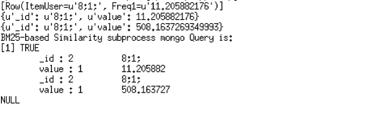
The results can then be queried in the Scala Spark-shell and in Spark applications.

The results can then be queried in the Scala Spark-shell and in Spark applications.
SparkR Application
In order to implement the first one set MapReduce using a Spark Pipe SparkR application and query the results in MongoDB (RMongoDB and PyMongo) the following arrangements should be made.
Input data file: InputData.txt (tab-separated)
Local system input data folder: < Local System Input Data Folder>
Local system input data folder: < Local System Input Data Folder>
Local system mapper file folder: < Local System
mapper File Folder >
Local system reducer file folder: < Local System
reducer File Folder >
Local system output data file folder: < Local
System Output Data Folder>
MongoDB instance: Have an instance of MongoDB with the arrangements in the MongoDB illustration
MongoDB instance: Have an instance of MongoDB with the arrangements in the MongoDB illustration
The MapReduce (and query) can be implemented using an application and a script file. The script (for the application and the supporting script) can be prepared using the tutorials in this post, this post, this post, this document, this post, this post, this post, this post, this post, this post, this post, this post and this post. The next step is to save the following SparkR application and SparkRApplicationScript files in appropriate local system folders.
The application can be run using the bin/spark-submit script.
These are the contents of the resulting output file/SQL query/NoSQL query.


Scala Spark-shell
The similarity measure MapReduce nine can be conducted using the Spark Pipe facility in a Scala Spark-shell program. The program can be complemented with MongoDB queries using RMongoDB and PyMongoDB. The first step is to make the following arrangements.
Input data file: InputData.txt (tab-separated)
Local system input data folder: < Local System
Input Data Folder>
Local system mapper file folder: < Local System
mapper File Folder >
Local system reducer file folder: < Local System
reducer File Folder >
Local system output data file folder: < Local
System Output Data Folder>
The next step is to save the following scripts in appropriate local system folders.
The next step is to run the following program prepared using the tutorials in this post, this post, this post, this post, this post, this guide and this post.
The next step is to run the following program prepared using the tutorials in this post, this post, this post, this post, this post, this guide and this post.
These are the contents of the resulting output file/SQL query/NoSQL query.


5. Query/Analyze the results
Once all the output data has been generated, one can conduct queries using MongoDB, a PySpark application, a SparkR application and a Java application. The BM25-based measures were calculated for user 8 and item 1. The queries using MongoDB, the Spark Pipe facility in a SparkR application (including RMongoDB) and the Spark Pipe facility in a Scala Spark-shell program were shown in the last section.
The three set TF-IDF Cosine-based Similarity measure query for user 8 and item 1 can be generated using a SparkR application prepared using the tutorials in this post, this post, this post, this document, this post, this post, this guide, this guide, this post, this post, this post and this post. The query can also be complemented with the one set MapReduce queries in MongoDB and PyMongo.
The first step is to make the following arrangements.
Input data file: InputData.txt (tab-separated)
In order to generate a query the following application file and application script file can be saved in local system folders.
The first step is to make the following arrangements.
Input data file: InputData.txt (tab-separated)
Local system input data folder: < Local System Input Data Folder>
Local system mapper file folder: < Local System mapper File Folder >
Local system reducer file folder: < Local System reducer File Folder >
Local system output data file folder: < Local System Output Data Folder>In order to generate a query the following application file and application script file can be saved in local system folders.
The application can be run using the bin/spark-submit script.
This will generate the following output.


The three set TF Cosine-based Similarity measure query for user 8 and item 1 can be generated using a Java application. This can be done by firstly appending the Java application code from the last section in line 110 and line 111 as follows.
The next step is to run the application (using the bin/spark-submit) with the input file for Similarity measure MapReduce three, four and five. This will generate the following output.
The three set TF-IDF Cosine-based Similarity measure query for user 8 and item 1 can be generated using a Java application with the appended code and using the input file for Similarity measure MapReduce six, seven and eight. The bin/spark-submit run will generate the following output.
The three set Okapi BM25 Cosine-based Similarity measure query for user 8 and item 1 can be generated using a Java application with the appended code and using the input file for Similarity measure MapReduce eleven, twelve and thirteen. The bin/spark-submit run will generate the following output.
The one set TF-IDF Cosine-based Similarity measure for user 8 and item 1 can be generated using a PySpark application. In order to implement the first one set MapReduce using a Spark Pipe PySpark application and query results in MongoDB (using RMongoDB and PyMongo) the following arrangements should be made.
Input data file: InputData.txt (tab-separated)
Local system input data folder: < Local System Input Data Folder>
Local system mapper file folder: < Local System mapper File Folder >
Local system reducer file folder: < Local System reducer File Folder >
Local system output data file folder: < Local System Output Data Folder>
MongoDB instance: Have an instance of MongoDB with the arrangements in the MongoDB illustration
The PySpark application script (and supporting file script) can be prepared using the tutorials in this post, this post, this post, this post, this post, this guide, this guide, this post and this post. The following PySpark application file (PySparkPipeOnesetApp.py) and PySpark Application script file (PySparkOneSetAppScript.R) can be saved in local system folders.
The next step is to use spark-submit to run the application..
This will generate the following output.

6. Conclusions
The post provided an illustration of how to implement the MapReduce programming model to the GroupLens HetRec 2011 dataset using the methodology outlined in Cantador, Bellogin and Vallet (2010). The approach can be further fine tuned to conduct the other analyses outlined in the paper.
Interested in other Big data analyses and Cloud computing resources from the Stats Cosmos blog?
Check out our other blog posts
Subscribe
to our RSS feeds for blog material updates
Or get a 28% discount to our exciting training opportunity bundle

Sources
http://bit.ly/1tusyEE
http://bit.ly/1Y07BPl
http://bit.ly/1rDzezL
http://bit.ly/1V5cK57
http://bit.ly/1RythtQ
http://bit.ly/1TAOH9I
http://bit.ly/1YxRLtN
http://bit.ly/1WSfBB5
http://bit.ly/1rtVawg
http://bit.ly/231JrU3
http://bit.ly/1Q5vX1t
http://bit.ly/1omcG4d
http://bit.ly/1TiHqjD
http://bit.ly/1Y08OWK
http://bit.ly/1M0oCUO
http://bit.ly/1PFIW8p
http://bit.ly/21TGWAx
http://bit.ly/1Uo1MH8
http://bit.ly/262B8Mv
http://bit.ly/1UTyEr2
http://bit.ly/1RKV5dQ
http://bit.ly/1W4xED9
http://bit.ly/21rwvVv
http://bit.ly/1OuZA19
http://bit.ly/1UFeOgy
http://bit.ly/262BQcE
http://bit.ly/1T76xr7
http://bit.ly/1UeusA6
http://bit.ly/268y3qY
http://bit.ly/1Ueuwjj
http://bit.ly/1sKO0oT
http://bit.ly/1Y07GTd
http://bit.ly/1QcuOe5
http://bit.ly/1UFf3IF
http://bit.ly/1Qc7Gc8
http://bit.ly/1WlCMnp
http://bit.ly/1NoLZIf
http://bit.ly/1tutIQq
http://bit.ly/1sKOIlR
http://bit.ly/1rtWuzr
http://ibm.co/1T3h0ml
http://bit.ly/1SZPyVw
http://bit.ly/1UgJ47t
http://bit.ly/21rwXDt
http://bit.ly/1Y09F9Z
http://bit.ly/1SN27EA
http://bit.ly/1WlCMnp
http://bit.ly/1Y08WFT
http://bit.ly/24WQCvF
http://bit.ly/1UBhVdw
http://bit.ly/1tuuFIF
http://bit.ly/1UezwnY
http://bit.ly/268CGRV
http://bit.ly/1UFi8bv
http://bit.ly/1tuxwkL
http://bit.ly/1Qcz518
http://bit.ly/1Ueuwjj
http://bit.ly/1QcuOe5
http://bit.ly/1sKRrMc
http://bit.ly/1UBka0r